Chapter 8 Regression Analysis
Regression analysis is the workhorse of empirical economics. It allows us to estimate relationships between variables, test hypotheses, and make predictions. This chapter introduces regression modeling in R, starting with ordinary least squares (OLS) for continuous outcomes, then moving to binary response models (logit and probit) for yes/no outcomes, and finally count data models (Poisson) for discrete counts.
library(tidyverse)

# Load all datasets
macro <- read_csv("data/us_macrodata.csv")
states <- read_csv("data/acs_state.csv")
pums <- read_csv("data/acs_pums.csv")
cafe <- read_csv("data/cafe_sales.csv")
8.1 Linear Regression with lm()
The lm() function fits linear models using ordinary least squares. The basic syntax is lm(y ~ x, data = df), where y is the dependent variable and x is the independent variable.
8.1.1 Simple Linear Regression
Let’s start with a simple regression examining how education levels relate to median household income across states.
# Simple linear regression: income as a function of education
model1 <- lm(median_household_income ~ bachelors_or_higher, data = states)

# View the results
summary(model1)
##
## Call:
## lm(formula = median_household_income ~ bachelors_or_higher, data = states)
##
## Residuals:
## Min 1Q Median 3Q Max
## -40859 -3531 -361 3573 19441
##
## Coefficients:
## Estimate Std. Error t value Pr(>|t|)
## (Intercept) 18807 6583 2.857 0.00622 **
## bachelors_or_higher 162940 19130 8.518 2.66e-11 ***
## ---
## Signif. codes: 0 '***' 0.001 '**' 0.01 '*' 0.05 '.' 0.1 ' ' 1
##
## Residual standard error: 9149 on 50 degrees of freedom
## Multiple R-squared: 0.592, Adjusted R-squared: 0.5838
## F-statistic: 72.55 on 1 and 50 DF, p-value: 2.66e-11The summary() output contains several important pieces of information:
- Coefficients: The intercept and slope estimates with their standard errors, t-statistics, and p-values
- R-squared: The proportion of variance in the dependent variable explained by the model
- F-statistic: Tests whether the model as a whole is statistically significant
The coefficient on bachelors_or_higher tells us that a one-unit increase in the bachelor’s degree rate (which is measured as a proportion, so 0.01 = 1 percentage point) is associated with approximately $1,100 higher median household income.
8.1.2 Extracting Model Components
R stores regression results as objects containing many useful components.
##         (Intercept) bachelors_or_higher
## 18806.87 162940.12## 1 2 3 4 5 6
## 63140.25 68908.16 70619.99 59062.12 77244.37 90061.73## 1 2 3 4 5 6
## -3531.249 17461.838 1961.008 -2727.124 14660.631 -2463.732## 2.5 % 97.5 %
## (Intercept) 5584.345 32029.39
## bachelors_or_higher 124517.006 201363.23## [1] 0.59200488.1.3 Visualizing the Regression Line
ggplot(states, aes(x = bachelors_or_higher, y = median_household_income)) +
  geom_point() +
  geom_smooth(method = "lm", se = TRUE) +
  scale_x_continuous(labels = scales::percent) +
  scale_y_continuous(labels = scales::dollar) +
  labs(
    title = "Education and Income Across U.S. States",
    x = "Percent with Bachelor's Degree or Higher",
    y = "Median Household Income"
  ) +
  theme_minimal()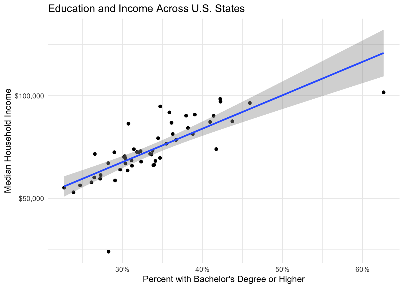
8.2 Multiple Linear Regression
Most economic questions involve multiple explanatory variables. The formula syntax in R uses + to add variables.
# Multiple regression: income as a function of education, unemployment, and homeownership
model2 <- lm(median_household_income ~ bachelors_or_higher + unemployment_rate +
               homeownership_rate, data = states)

summary(model2)
##
## Call:
## lm(formula = median_household_income ~ bachelors_or_higher +
## unemployment_rate + homeownership_rate, data = states)
##
## Residuals:
## Min 1Q Median 3Q Max
## -17400.5 -4300.6 -624.6 3947.8 19605.7
##
## Coefficients:
## Estimate Std. Error t value Pr(>|t|)
## (Intercept) 70505 23678 2.978 0.00454 **
## bachelors_or_higher 142070 20292 7.001 7.32e-09 ***
## unemployment_rate -325676 77262 -4.215 0.00011 ***
## homeownership_rate -42013 25937 -1.620 0.11183
## ---
## Signif. codes: 0 '***' 0.001 '**' 0.01 '*' 0.05 '.' 0.1 ' ' 1
##
## Residual standard error: 7977 on 48 degrees of freedom
## Multiple R-squared: 0.7022, Adjusted R-squared: 0.6836
## F-statistic: 37.74 on 3 and 48 DF, p-value: 1.118e-128.2.2 Example: The Mincer Wage Equation
The Mincer equation is a classic specification in labor economics that relates wages to education and experience. Let’s estimate it using the PUMS data.
# Prepare the data
pums_workers <- pums %>%
  filter(wage_income > 0, !is.na(education), age >= 18, age <= 65) %>%
  mutate(
    log_wage = log(wage_income),
    # Create years of education from categories
    years_education = case_when(
      education == "Less than HS" ~ 10,
      education == "High school" ~ 12,
      education == "Some college" ~ 14,
      education == "Bachelors" ~ 16,
      education == "Masters" ~ 18,
      education == "Professional/Doctorate" ~ 20
    ),
    # Approximate experience as age - education - 6
    experience = age - years_education - 6,
    experience_sq = experience^2
  )

# Estimate the Mincer equation
mincer <- lm(log_wage ~ years_education + experience + experience_sq,
             data = pums_workers)

summary(mincer)
##
## Call:
## lm(formula = log_wage ~ years_education + experience + experience_sq,
## data = pums_workers)
##
## Residuals:
## Min 1Q Median 3Q Max
## -8.8923 -0.4142 0.1706 0.6404 4.2614
##
## Coefficients:
## Estimate Std. Error t value Pr(>|t|)
## (Intercept) 7.048e+00 6.535e-02 107.85 <2e-16 ***
## years_education 1.738e-01 4.223e-03 41.15 <2e-16 ***
## experience 9.640e-02 2.811e-03 34.30 <2e-16 ***
## experience_sq -1.688e-03 6.339e-05 -26.62 <2e-16 ***
## ---
## Signif. codes: 0 '***' 0.001 '**' 0.01 '*' 0.05 '.' 0.1 ' ' 1
##
## Residual standard error: 1.063 on 10759 degrees of freedom
## Multiple R-squared: 0.2477, Adjusted R-squared: 0.2475
## F-statistic: 1181 on 3 and 10759 DF, p-value: < 2.2e-16Interpretation:
- The coefficient on
years_educationrepresents the approximate percentage increase in wages for each additional year of education (about 10% per year) - The coefficients on experience and experience-squared capture the concave experience-earnings profile
8.2.3 Categorical Variables (Factor Variables)
R automatically creates dummy variables for factors. Let’s include education categories and sex in the wage equation.
# Using categorical education
pums_workers <- pums_workers %>%
  mutate(education = factor(education, levels = c("Less than HS",
                                                   "High school",
                                                   "Some college",
                                                   "Bachelors",
                                                   "Masters",
                                                   "Professional/Doctorate")))

model_categorical <- lm(log_wage ~ education + experience + experience_sq + sex,
                        data = pums_workers)

summary(model_categorical)
##
## Call:
## lm(formula = log_wage ~ education + experience + experience_sq +
## sex, data = pums_workers)
##
## Residuals:
## Min 1Q Median 3Q Max
## -8.8378 -0.3987 0.1763 0.6254 4.2056
##
## Coefficients:
## Estimate Std. Error t value Pr(>|t|)
## (Intercept) 8.625e+00 4.574e-02 188.58 < 2e-16 ***
## educationHigh school 3.405e-01 4.203e-02 8.10 6.09e-16 ***
## educationSome college 5.352e-01 4.104e-02 13.04 < 2e-16 ***
## educationBachelors 1.163e+00 4.195e-02 27.73 < 2e-16 ***
## educationMasters 1.392e+00 4.789e-02 29.06 < 2e-16 ***
## educationProfessional/Doctorate 1.633e+00 6.184e-02 26.41 < 2e-16 ***
## experience 9.450e-02 2.763e-03 34.21 < 2e-16 ***
## experience_sq -1.641e-03 6.224e-05 -26.37 < 2e-16 ***
## sexMale 3.717e-01 2.026e-02 18.35 < 2e-16 ***
## ---
## Signif. codes: 0 '***' 0.001 '**' 0.01 '*' 0.05 '.' 0.1 ' ' 1
##
## Residual standard error: 1.042 on 10754 degrees of freedom
## Multiple R-squared: 0.2776, Adjusted R-squared: 0.2771
## F-statistic: 516.7 on 8 and 10754 DF, p-value: < 2.2e-16The first category (“Less than HS”) is the reference group. Coefficients represent the difference in log wages relative to this group.
8.3 Diagnostic Plots
Regression assumptions should be checked using diagnostic plots.
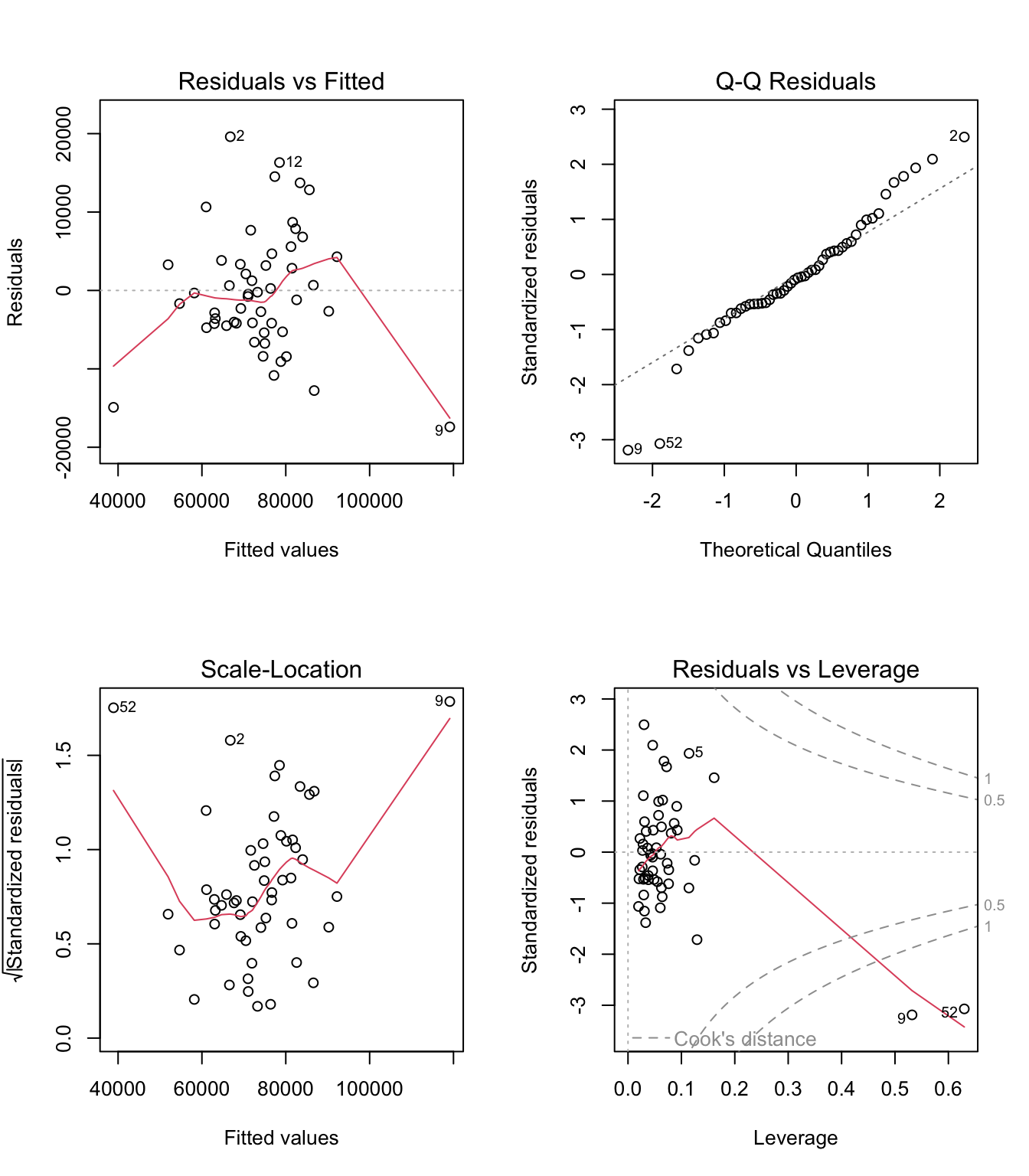
The four plots show:
- Residuals vs Fitted: Should show no pattern (tests linearity and homoskedasticity)
- Q-Q Plot: Points should follow the diagonal line (tests normality of residuals)
- Scale-Location: Should show horizontal band (tests homoskedasticity)
- Residuals vs Leverage: Identifies influential observations
8.3.1 Creating Custom Diagnostic Plots
# Add fitted values and residuals to data
states_diag <- states %>%
  filter(!is.na(median_household_income)) %>%
  mutate(
    fitted = fitted(model2),
    residuals = residuals(model2)
  )

# Residuals vs fitted plot with ggplot
ggplot(states_diag, aes(x = fitted, y = residuals)) +
  geom_point() +
  geom_hline(yintercept = 0, linetype = "dashed", color = "red") +
  geom_smooth(method = "loess", se = FALSE, color = "blue") +
  labs(title = "Residuals vs Fitted Values",
       x = "Fitted Values", y = "Residuals") +
  theme_minimal()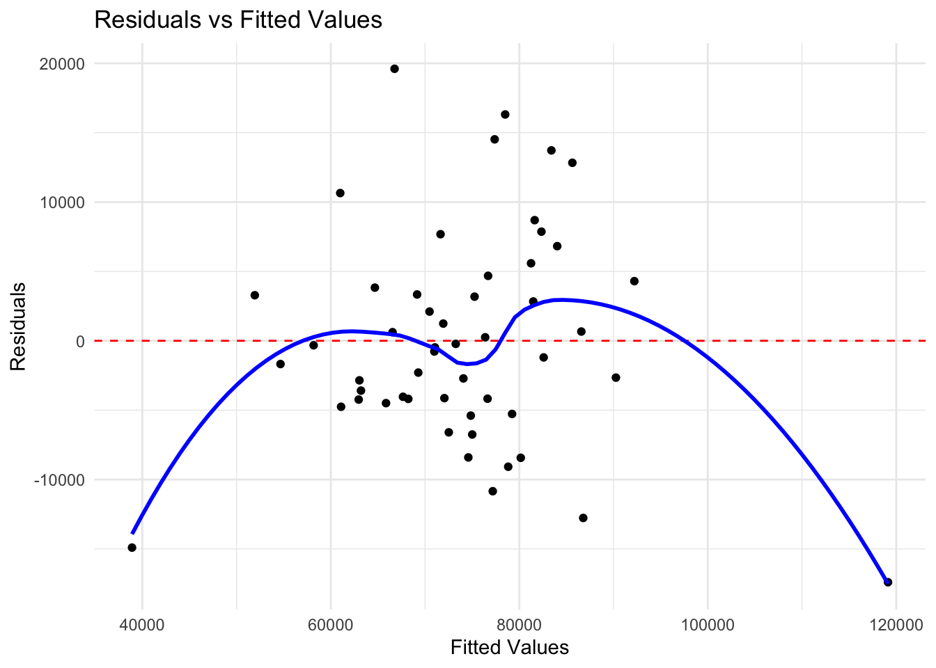
8.4 Robust Standard Errors
In the presence of heteroskedasticity, standard errors from OLS are biased. The sandwich and lmtest packages provide robust standard errors.
##
## t test of coefficients:
##
##                     Estimate Std. Error t value  Pr(>|t|)
## (Intercept)            70505      23678  2.9776 0.0045435 **
## bachelors_or_higher   142070      20292  7.0013 7.319e-09 ***
## unemployment_rate    -325676      77262 -4.2152 0.0001096 ***
## homeownership_rate    -42013      25937 -1.6198 0.1118263
## ---
## Signif. codes:  0 '***' 0.001 '**' 0.01 '*' 0.05 '.' 0.1 ' ' 1
# Heteroskedasticity-robust standard errors (HC1, similar to Stata)
coeftest(model2, vcov = vcovHC(model2, type = "HC1"))##
## t test of coefficients:
##
## Estimate Std. Error t value Pr(>|t|)
## (Intercept) 70505 30194 2.3351 0.02377 *
## bachelors_or_higher 142070 24853 5.7165 6.775e-07 ***
## unemployment_rate -325676 124635 -2.6130 0.01195 *
## homeownership_rate -42013 35604 -1.1800 0.24381
## ---
## Signif. codes: 0 '***' 0.001 '**' 0.01 '*' 0.05 '.' 0.1 ' ' 18.5 Binary Response Models: Logit and Probit
When the dependent variable is binary (0 or 1), linear regression is inappropriate. Logit and probit models constrain predicted probabilities to lie between 0 and 1.
8.5.1 The glm() Function
The glm() function fits generalized linear models, including logit and probit.
# Prepare employment data
pums_employment <- pums %>%
  filter(age >= 25, age <= 55, !is.na(education), !is.na(sex), !is.na(employed)) %>%
  mutate(
    employed = as.integer(employed == 1),
    # Recode education to simpler categories
    education_cat = case_when(
      education == "Less than HS" ~ "Less than HS",
      education == "High school" ~ "High school",
      education == "Some college" ~ "Some college",
      education == "Bachelors" ~ "Bachelor's+",
      education %in% c("Masters", "Professional/Doctorate") ~ "Bachelor's+"
    ),
    education_cat = factor(education_cat, levels = c("Less than HS",
                                                      "High school",
                                                      "Some college",
                                                      "Bachelor's+"))
  )

# Logit model: probability of employment
logit_model <- glm(employed ~ education_cat + age + sex,
                   family = binomial(link = "logit"),
                   data = pums_employment)

summary(logit_model)
##
## Call:
## glm(formula = employed ~ education_cat + age + sex, family = binomial(link = "logit"),
## data = pums_employment)
##
## Coefficients:
## Estimate Std. Error z value Pr(>|z|)
## (Intercept) -2.657e+01 2.132e+04 -0.001 0.999
## education_catHigh school 5.410e-13 1.400e+04 0.000 1.000
## education_catSome college 1.977e-14 1.365e+04 0.000 1.000
## education_catBachelor's+ 3.454e-14 1.301e+04 0.000 1.000
## age -3.976e-18 4.136e+02 0.000 1.000
## sexMale 2.156e-13 7.464e+03 0.000 1.000
##
## (Dispersion parameter for binomial family taken to be 1)
##
## Null deviance: 0.000e+00 on 9262 degrees of freedom
## Residual deviance: 5.374e-08 on 9257 degrees of freedom
## AIC: 12
##
## Number of Fisher Scoring iterations: 258.5.2 Probit Model
# Probit model (same specification)
probit_model <- glm(employed ~ education_cat + age + sex,
                    family = binomial(link = "probit"),
                    data = pums_employment)

summary(probit_model)
##
## Call:
## glm(formula = employed ~ education_cat + age + sex, family = binomial(link = "probit"),
## data = pums_employment)
##
## Coefficients:
## Estimate Std. Error z value Pr(>|z|)
## (Intercept) -6.991e+00 4.430e+03 -0.002 0.999
## education_catHigh school 2.318e-13 2.908e+03 0.000 1.000
## education_catSome college 1.238e-14 2.836e+03 0.000 1.000
## education_catBachelor's+ 1.647e-14 2.702e+03 0.000 1.000
## age -5.071e-19 8.591e+01 0.000 1.000
## sexMale 8.978e-14 1.551e+03 0.000 1.000
##
## (Dispersion parameter for binomial family taken to be 1)
##
## Null deviance: 0.0000e+00 on 9262 degrees of freedom
## Residual deviance: 2.5241e-08 on 9257 degrees of freedom
## AIC: 12
##
## Number of Fisher Scoring iterations: 258.5.3 Interpreting Coefficients
Logit coefficients are in log-odds. To interpret them as odds ratios, exponentiate:
##               (Intercept)  education_catHigh school education_catSome college
##             -2.656607e+01              5.409722e-13              1.976718e-14
##  education_catBachelor's+                       age                   sexMale
## 3.453892e-14 -3.976407e-18 2.156117e-13## (Intercept) education_catHigh school education_catSome college
## 2.900701e-12 1.000000e+00 1.000000e+00
## education_catBachelor's+ age sexMale
## 1.000000e+00 1.000000e+00 1.000000e+00# Odds ratios with confidence intervals (using Wald CIs for stability)
ci <- confint.default(logit_model)
exp(cbind(OR = coef(logit_model), ci))## OR 2.5 % 97.5 %
## (Intercept) 2.900701e-12 0 Inf
## education_catHigh school 1.000000e+00 0 Inf
## education_catSome college 1.000000e+00 0 Inf
## education_catBachelor's+ 1.000000e+00 0 Inf
## age 1.000000e+00 0 Inf
## sexMale 1.000000e+00 0 InfAn odds ratio greater than 1 means higher odds of employment; less than 1 means lower odds.
8.5.4 Marginal Effects
For more intuitive interpretation, calculate marginal effects (the change in probability for a unit change in x). The margins package makes this easy.
library(margins)

# Average marginal effects
margins_logit <- margins(logit_model)
summary(margins_logit)
## factor AME SE z p lower upper
## age 0.0000 0.0000 0.0000 1.0000 -0.0000 0.0000
## education_catBachelor's+ 0.0000 0.0000 0.0000 1.0000 -0.0000 0.0000
## education_catHigh school 0.0000 0.0000 0.0000 1.0000 -0.0000 0.0000
## education_catSome college 0.0000 0.0000 0.0000 1.0000 -0.0000 0.0000
## sexMale 0.0000 0.0000 0.0000 1.0000 -0.0000 0.0000The marginal effect tells us the percentage point change in the probability of employment for a one-unit change in the explanatory variable.
8.5.5 Predicted Probabilities
# Create prediction data
new_data <- expand.grid(
  education_cat = levels(pums_employment$education_cat),
  age = 40,
  sex = c("Male", "Female")
)

# Predict probabilities
new_data$predicted_prob <- predict(logit_model, newdata = new_data, type = "response")

# Display
new_data %>%
  pivot_wider(names_from = sex, values_from = predicted_prob) %>%
  mutate(across(c(Male, Female), ~scales::percent(.x, accuracy = 0.1)))
## # A tibble: 4 × 4
## education_cat age Male Female
## <fct> <dbl> <chr> <chr>
## 1 Less than HS 40 0.0% 0.0%
## 2 High school 40 0.0% 0.0%
## 3 Some college 40 0.0% 0.0%
## 4 Bachelor's+ 40 0.0% 0.0%8.5.6 Visualizing Predicted Probabilities
# Predict across age range
pred_data <- expand.grid(
  education_cat = c("High school", "Bachelor's+"),
  age = seq(25, 55, by = 1),
  sex = "Female"
)

pred_data$prob <- predict(logit_model, newdata = pred_data, type = "response")

ggplot(pred_data, aes(x = age, y = prob, color = education_cat)) +
  geom_line(linewidth = 1) +
  scale_y_continuous(labels = scales::percent, limits = c(0.5, 1)) +
  labs(
    title = "Predicted Probability of Employment by Age and Education",
    subtitle = "Female workers",
    x = "Age",
    y = "Probability of Employment",
    color = "Education"
  ) +
  theme_minimal()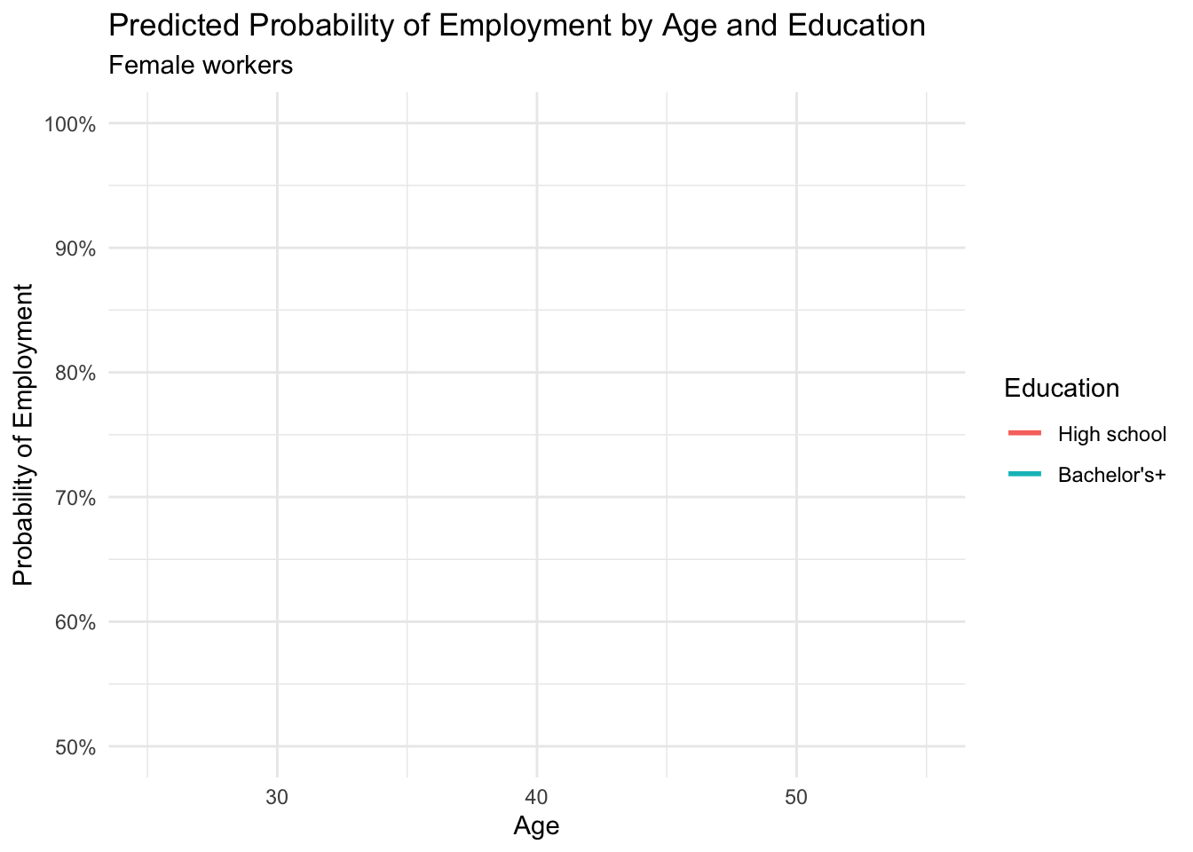
8.5.7 Model Fit for Binary Models
## 'log Lik.' -2.68692e-08 (df=6)## [1] 12## [1] 54.8027## df AIC
## logit_model 6 12
## probit_model 6 12# Pseudo R-squared (McFadden's)
null_model <- glm(employed ~ 1, family = binomial, data = pums_employment)
1 - logLik(logit_model) / logLik(null_model)## 'log Lik.' 8.263909e-09 (df=6)8.6 Count Data Models: Poisson Regression
When the dependent variable is a count (0, 1, 2, …), Poisson regression is appropriate. The model assumes the count follows a Poisson distribution with mean that depends on the explanatory variables.
8.6.1 Preparing Count Data
Let’s analyze daily transaction counts at the cafe.
# Aggregate to daily counts
cafe_daily <- cafe %>%
  group_by(date, year, month, day_of_week) %>%
  summarize(
    transactions = n(),
    revenue = sum(price),
    .groups = "drop"
  ) %>%
  mutate(
    weekend = day_of_week %in% c("Sat", "Sun"),
    covid_period = date >= "2020-03-01" & date <= "2020-12-31",
    day_of_week = factor(day_of_week,
                         levels = c("Mon", "Tue", "Wed", "Thu", "Fri", "Sat", "Sun"))
  )

head(cafe_daily)
## # A tibble: 6 × 8
## date year month day_of_week transactions revenue weekend covid_period
## <date> <dbl> <dbl> <fct> <int> <dbl> <lgl> <lgl>
## 1 2019-01-01 2019 1 Tue 307 1169 FALSE FALSE
## 2 2019-01-02 2019 1 Wed 296 1122. FALSE FALSE
## 3 2019-01-03 2019 1 Thu 257 964. FALSE FALSE
## 4 2019-01-04 2019 1 Fri 240 894. FALSE FALSE
## 5 2019-01-05 2019 1 Sat 368 1388. TRUE FALSE
## 6 2019-01-06 2019 1 Sun 379 1473. TRUE FALSE## Min. 1st Qu. Median Mean 3rd Qu. Max.
## 53.0 235.2 269.0 268.3 303.0 469.0# Distribution of counts
ggplot(cafe_daily, aes(x = transactions)) +
geom_histogram(binwidth = 10, fill = "steelblue", color = "white") +
labs(title = "Distribution of Daily Transaction Counts",
x = "Number of Transactions", y = "Frequency") +
theme_minimal()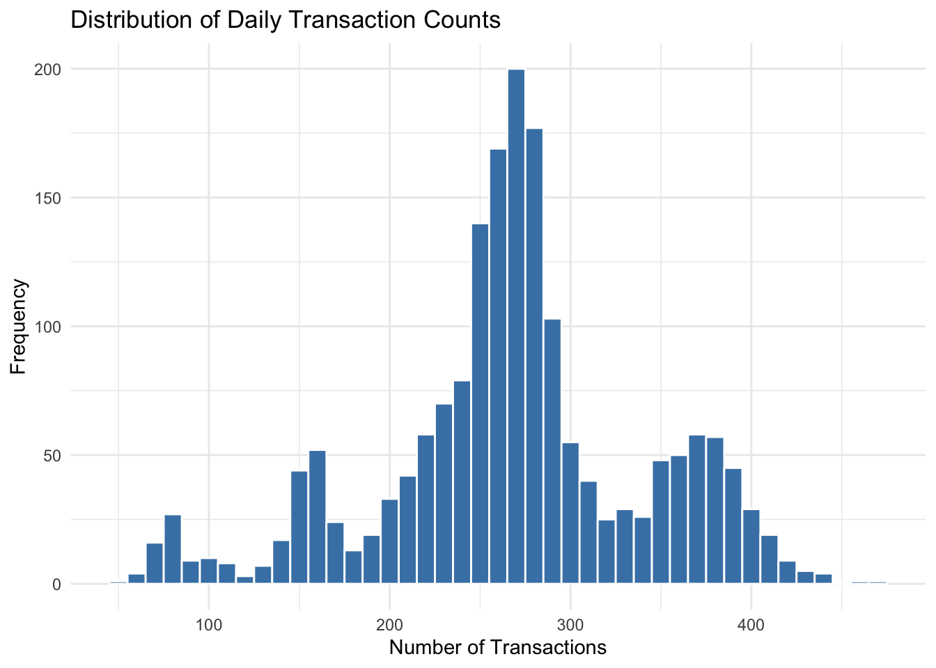
8.6.2 Fitting a Poisson Model
# Poisson regression
poisson_model <- glm(transactions ~ day_of_week + year + covid_period,
                     family = poisson(link = "log"),
                     data = cafe_daily)

summary(poisson_model)
##
## Call:
## glm(formula = transactions ~ day_of_week + year + covid_period,
## family = poisson(link = "log"), data = cafe_daily)
##
## Coefficients:
## Estimate Std. Error z value Pr(>|z|)
## (Intercept) -35.093789 2.079157 -16.879 <2e-16 ***
## day_of_weekTue -0.007864 0.005629 -1.397 0.1624
## day_of_weekWed -0.007279 0.005628 -1.293 0.1959
## day_of_weekThu -0.005266 0.005625 -0.936 0.3492
## day_of_weekFri -0.011505 0.005631 -2.043 0.0411 *
## day_of_weekSat 0.316169 0.005222 60.547 <2e-16 ***
## day_of_weekSun 0.318675 0.005221 61.037 <2e-16 ***
## year 0.020121 0.001029 19.561 <2e-16 ***
## covid_periodTRUE -0.598633 0.004986 -120.066 <2e-16 ***
## ---
## Signif. codes: 0 '***' 0.001 '**' 0.01 '*' 0.05 '.' 0.1 ' ' 1
##
## (Dispersion parameter for poisson family taken to be 1)
##
## Null deviance: 40698.3 on 1825 degrees of freedom
## Residual deviance: 9097.6 on 1817 degrees of freedom
## AIC: 22596
##
## Number of Fisher Scoring iterations: 48.6.3 Interpreting Poisson Coefficients
Poisson coefficients represent the change in the log of expected counts. Exponentiating gives the multiplicative effect (incidence rate ratio).
##      (Intercept)   day_of_weekTue   day_of_weekWed   day_of_weekThu
##    -35.093789108     -0.007864462     -0.007278799     -0.005266263
##   day_of_weekFri   day_of_weekSat   day_of_weekSun             year
##     -0.011504841      0.316169000      0.318675297      0.020121263
## covid_periodTRUE
## -0.598632580## (Intercept) day_of_weekTue day_of_weekWed day_of_weekThu
## 5.740650e-16 9.921664e-01 9.927476e-01 9.947476e-01
## day_of_weekFri day_of_weekSat day_of_weekSun year
## 9.885611e-01 1.371862e+00 1.375305e+00 1.020325e+00
## covid_periodTRUE
## 5.495626e-01## IRR 2.5 % 97.5 %
## (Intercept) 5.740650e-16 9.746230e-18 3.375990e-14
## day_of_weekTue 9.921664e-01 9.812804e-01 1.003173e+00
## day_of_weekWed 9.927476e-01 9.818570e-01 1.003759e+00
## day_of_weekThu 9.947476e-01 9.838405e-01 1.005776e+00
## day_of_weekFri 9.885611e-01 9.777101e-01 9.995324e-01
## day_of_weekSat 1.371862e+00 1.357897e+00 1.385979e+00
## day_of_weekSun 1.375305e+00 1.361307e+00 1.389454e+00
## year 1.020325e+00 1.018270e+00 1.022385e+00
## covid_periodTRUE 5.495626e-01 5.442124e-01 5.549533e-01An IRR of 1.15 means the expected count is 15% higher; an IRR of 0.80 means 20% lower.
8.6.4 Predicted Counts
# Predict expected counts for each day of week
pred_days <- data.frame(
  day_of_week = factor(c("Mon", "Tue", "Wed", "Thu", "Fri", "Sat", "Sun"),
                       levels = levels(cafe_daily$day_of_week)),
  year = 2023,
  covid_period = FALSE
)

pred_days$expected_count <- predict(poisson_model, newdata = pred_days, type = "response")

pred_days %>%
  select(day_of_week, expected_count) %>%
  mutate(expected_count = round(expected_count, 0))
## day_of_week expected_count
## 1 Mon 274
## 2 Tue 271
## 3 Wed 272
## 4 Thu 272
## 5 Fri 270
## 6 Sat 375
## 7 Sun 3768.6.5 Overdispersion
A key assumption of Poisson regression is that the mean equals the variance. When the variance exceeds the mean (overdispersion), standard errors are underestimated. Check for this:
# Dispersion statistic (should be close to 1 for Poisson)
dispersion <- sum(residuals(poisson_model, type = "pearson")^2) / poisson_model$df.residual
dispersion
## [1] 4.871176If dispersion is substantially greater than 1, consider using quasi-Poisson or negative binomial regression:
# Quasi-Poisson (adjusts standard errors for overdispersion)
quasi_model <- glm(transactions ~ day_of_week + year + covid_period,
                   family = quasipoisson(link = "log"),
                   data = cafe_daily)

summary(quasi_model)
##
## Call:
## glm(formula = transactions ~ day_of_week + year + covid_period,
## family = quasipoisson(link = "log"), data = cafe_daily)
##
## Coefficients:
## Estimate Std. Error t value Pr(>|t|)
## (Intercept) -35.093789 4.588854 -7.648 3.3e-14 ***
## day_of_weekTue -0.007864 0.012424 -0.633 0.527
## day_of_weekWed -0.007279 0.012421 -0.586 0.558
## day_of_weekThu -0.005266 0.012415 -0.424 0.671
## day_of_weekFri -0.011505 0.012429 -0.926 0.355
## day_of_weekSat 0.316169 0.011525 27.433 < 2e-16 ***
## day_of_weekSun 0.318675 0.011523 27.655 < 2e-16 ***
## year 0.020121 0.002270 8.863 < 2e-16 ***
## covid_periodTRUE -0.598633 0.011004 -54.400 < 2e-16 ***
## ---
## Signif. codes: 0 '***' 0.001 '**' 0.01 '*' 0.05 '.' 0.1 ' ' 1
##
## (Dispersion parameter for quasipoisson family taken to be 4.871179)
##
## Null deviance: 40698.3 on 1825 degrees of freedom
## Residual deviance: 9097.6 on 1817 degrees of freedom
## AIC: NA
##
## Number of Fisher Scoring iterations: 48.6.6 Negative Binomial Regression
For more severe overdispersion, negative binomial regression is preferred. It requires the MASS package.
library(MASS)

# Negative binomial regression
negbin_model <- glm.nb(transactions ~ day_of_week + year + covid_period,
                       data = cafe_daily)

summary(negbin_model)
##
## Call:
## glm.nb(formula = transactions ~ day_of_week + year + covid_period,
## data = cafe_daily, init.theta = 52.9606772, link = log)
##
## Coefficients:
## Estimate Std. Error z value Pr(>|z|)
## (Intercept) -34.101470 5.281566 -6.457 1.07e-10 ***
## day_of_weekTue -0.007332 0.013340 -0.550 0.583
## day_of_weekWed -0.008286 0.013341 -0.621 0.535
## day_of_weekThu -0.004623 0.013339 -0.347 0.729
## day_of_weekFri -0.012644 0.013342 -0.948 0.343
## day_of_weekSat 0.315146 0.013169 23.932 < 2e-16 ***
## day_of_weekSun 0.317045 0.013169 24.075 < 2e-16 ***
## year 0.019631 0.002613 7.512 5.80e-14 ***
## covid_periodTRUE -0.598171 0.010377 -57.646 < 2e-16 ***
## ---
## Signif. codes: 0 '***' 0.001 '**' 0.01 '*' 0.05 '.' 0.1 ' ' 1
##
## (Dispersion parameter for Negative Binomial(52.9607) family taken to be 1)
##
## Null deviance: 7529.7 on 1825 degrees of freedom
## Residual deviance: 1983.2 on 1817 degrees of freedom
## AIC: 18723
##
## Number of Fisher Scoring iterations: 1
##
##
## Theta: 52.96
## Std. Err.: 2.29
##
## 2 x log-likelihood: -18702.628.7 Comparing Models
8.7.1 Nested Model Comparison with Likelihood Ratio Tests
# Restricted model (no day of week effects)
poisson_restricted <- glm(transactions ~ year + covid_period,
                          family = poisson(link = "log"),
                          data = cafe_daily)

# Likelihood ratio test
anova(poisson_restricted, poisson_model, test = "LRT")
## Analysis of Deviance Table
##
## Model 1: transactions ~ year + covid_period
## Model 2: transactions ~ day_of_week + year + covid_period
## Resid. Df Resid. Dev Df Deviance Pr(>Chi)
## 1 1823 20486.6
## 2 1817 9097.6 6 11389 < 2.2e-16 ***
## ---
## Signif. codes: 0 '***' 0.001 '**' 0.01 '*' 0.05 '.' 0.1 ' ' 18.8 Presenting Regression Results
8.8.1 Creating Regression Tables
The broom package converts regression output to tidy data frames.
## # A tibble: 4 × 5
##   term                estimate std.error statistic       p.value
##   <chr>                  <dbl>     <dbl>     <dbl>         <dbl>
## 1 (Intercept)           70505.    23678.      2.98 0.00454
## 2 bachelors_or_higher  142070.    20292.      7.00 0.00000000732
## 3 unemployment_rate   -325676.    77262.     -4.22 0.000110
## 4 homeownership_rate -42013. 25937. -1.62 0.112## # A tibble: 1 × 12
## r.squared adj.r.squared sigma statistic p.value df logLik AIC BIC
## <dbl> <dbl> <dbl> <dbl> <dbl> <dbl> <dbl> <dbl> <dbl>
## 1 0.702 0.684 7977. 37.7 1.12e-12 3 -539. 1088. 1098.
## # ℹ 3 more variables: deviance <dbl>, df.residual <int>, nobs <int>## # A tibble: 6 × 10
## median_household_income bachelors_or_higher unemployment_rate
## <dbl> <dbl> <dbl>
## 1 59609 0.272 0.0512
## 2 86370 0.307 0.0601
## 3 72581 0.318 0.0533
## 4 56335 0.247 0.0513
## 5 91905 0.359 0.0636
## 6 87598 0.437 0.0448
## # ℹ 7 more variables: homeownership_rate <dbl>, .fitted <dbl>, .resid <dbl>,
## # .hat <dbl>, .sigma <dbl>, .cooksd <dbl>, .std.resid <dbl>8.8.2 Publication-Quality Tables with gt
library(gt)

# Create a nice coefficient table
tidy(model2, conf.int = TRUE) %>%
  mutate(
    term = case_when(
      term == "(Intercept)" ~ "Constant",
      term == "bachelors_or_higher" ~ "Bachelor's Degree Rate",
      term == "unemployment_rate" ~ "Unemployment Rate",
      term == "homeownership_rate" ~ "Homeownership Rate"
    )
  ) %>%
  gt() %>%
  tab_header(
    title = "Determinants of State Median Household Income",
    subtitle = "OLS Regression Results"
  ) %>%
  fmt_number(columns = c(estimate, std.error, statistic, conf.low, conf.high),
             decimals = 2) %>%
  fmt_number(columns = p.value, decimals = 4) %>%
  cols_label(
    term = "Variable",
    estimate = "Coefficient",
    std.error = "Std. Error",
    statistic = "t-statistic",
    p.value = "p-value",
    conf.low = "95% CI Low",
    conf.high = "95% CI High"
)| Determinants of State Median Household Income | ||||||
| OLS Regression Results | ||||||
| Variable | Coefficient | Std. Error | t-statistic | p-value | 95% CI Low | 95% CI High |
|---|---|---|---|---|---|---|
| Constant | 70,504.77 | 23,678.50 | 2.98 | 0.0045 | 22,895.96 | 118,113.59 |
| Bachelor's Degree Rate | 142,070.15 | 20,291.97 | 7.00 | 0.0000 | 101,270.41 | 182,869.89 |
| Unemployment Rate | −325,676.29 | 77,261.91 | −4.22 | 0.0001 | −481,021.78 | −170,330.80 |
| Homeownership Rate | −42,012.77 | 25,936.91 | −1.62 | 0.1118 | −94,162.42 | 10,136.89 |
8.8.3 Comparing Multiple Models
# Multiple models for comparison
model_a <- lm(median_household_income ~ bachelors_or_higher, data = states)
model_b <- lm(median_household_income ~ bachelors_or_higher + unemployment_rate, data = states)
model_c <- lm(median_household_income ~ bachelors_or_higher + unemployment_rate +
                homeownership_rate, data = states)

# Combine results
comparison_df <- bind_rows(
  tidy(model_a) %>% mutate(model = "Model 1"),
  tidy(model_b) %>% mutate(model = "Model 2"),
  tidy(model_c) %>% mutate(model = "Model 3")
) %>%
  filter(term != "(Intercept)")

comparison_df %>%
  dplyr::select(model, term, estimate, std.error, p.value) %>%
  pivot_wider(
    names_from = model,
    values_from = c(estimate, std.error, p.value)
  )
## # A tibble: 3 × 10
## term `estimate_Model 1` `estimate_Model 2` `estimate_Model 3`
## <chr> <dbl> <dbl> <dbl>
## 1 bachelors_or_higher 162940. 160769. 142070.
## 2 unemployment_rate NA -279394. -325676.
## 3 homeownership_rate NA NA -42013.
## # ℹ 6 more variables: `std.error_Model 1` <dbl>, `std.error_Model 2` <dbl>,
## # `std.error_Model 3` <dbl>, `p.value_Model 1` <dbl>,
## # `p.value_Model 2` <dbl>, `p.value_Model 3` <dbl>8.9 Example: Phillips Curve Estimation
The Phillips curve describes the relationship between unemployment and inflation. Let’s estimate it using the macro data.
# Prepare data
macro_phillips <- macro %>%
  filter(year >= 1960) %>%
  mutate(
    inflation_pct = inflation * 100,
    unemployment_pct = unemployment * 100
  )

# Simple Phillips curve
phillips1 <- lm(inflation_pct ~ unemployment_pct, data = macro_phillips)
summary(phillips1)
##
## Call:
## lm(formula = inflation_pct ~ unemployment_pct, data = macro_phillips)
##
## Residuals:
## Min 1Q Median 3Q Max
## -4.3067 -1.5412 -0.5412 0.6502 10.0760
##
## Coefficients:
## Estimate Std. Error t value Pr(>|t|)
## (Intercept) 2.5843 1.3115 1.971 0.0532 .
## unemployment_pct 0.1914 0.2100 0.911 0.3657
## ---
## Signif. codes: 0 '***' 0.001 '**' 0.01 '*' 0.05 '.' 0.1 ' ' 1
##
## Residual standard error: 2.738 on 63 degrees of freedom
## Multiple R-squared: 0.01301, Adjusted R-squared: -0.00266
## F-statistic: 0.8302 on 1 and 63 DF, p-value: 0.3657# Plot
ggplot(macro_phillips, aes(x = unemployment_pct, y = inflation_pct)) +
geom_point(alpha = 0.6) +
geom_smooth(method = "lm", se = TRUE) +
labs(
title = "The Phillips Curve (1960-Present)",
x = "Unemployment Rate (%)",
y = "Inflation Rate (%)"
) +
theme_minimal()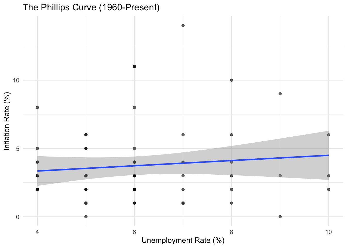
The simple Phillips curve shows a weak negative relationship. Let’s explore whether this relationship has changed over time.
# Phillips curve by era
macro_phillips <- macro_phillips %>%
  mutate(era = case_when(
    year < 1980 ~ "1960-1979",
    year < 2000 ~ "1980-1999",
    TRUE ~ "2000-Present"
  ))

ggplot(macro_phillips, aes(x = unemployment_pct, y = inflation_pct, color = era)) +
  geom_point(alpha = 0.6) +
  geom_smooth(method = "lm", se = FALSE) +
  labs(
    title = "The Phillips Curve by Era",
    x = "Unemployment Rate (%)",
    y = "Inflation Rate (%)",
    color = "Period"
  ) +
  theme_minimal()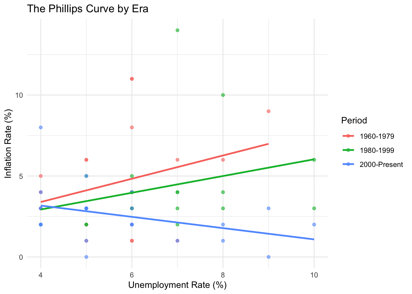
8.10 Example: Wage Determinants with PUMS
Let’s build a more complete wage equation including multiple factors.
# Comprehensive wage regression
wage_model <- lm(log_wage ~ education + experience + experience_sq + sex +
                   hours_worked + state,
                 data = pums_workers)

# Summary (showing just key coefficients)
tidy(wage_model) %>%
  filter(!str_starts(term, "state")) %>%
  gt() %>%
  tab_header(title = "Log Wage Regression Results") %>%
  fmt_number(columns = c(estimate, std.error, statistic), decimals = 3) %>%
fmt_number(columns = p.value, decimals = 4)| Log Wage Regression Results | ||||
| term | estimate | std.error | statistic | p.value |
|---|---|---|---|---|
| (Intercept) | 7.527 | 0.049 | 154.546 | 0.0000 |
| educationHigh school | 0.254 | 0.037 | 6.821 | 0.0000 |
| educationSome college | 0.452 | 0.036 | 12.450 | 0.0000 |
| educationBachelors | 0.950 | 0.037 | 25.450 | 0.0000 |
| educationMasters | 1.154 | 0.043 | 27.088 | 0.0000 |
| educationProfessional/Doctorate | 1.313 | 0.055 | 23.874 | 0.0000 |
| experience | 0.066 | 0.002 | 26.467 | 0.0000 |
| experience_sq | −0.001 | 0.000 | −19.732 | 0.0000 |
| sexMale | 0.193 | 0.018 | 10.619 | 0.0000 |
| hours_worked | 0.043 | 0.001 | 54.623 | 0.0000 |
8.11 Example: State Poverty Analysis
What factors predict poverty rates across states?
# Poverty rate determinants
poverty_model <- lm(poverty_rate ~ bachelors_or_higher + unemployment_rate +
                      median_age + homeownership_rate,
                    data = states %>% filter(state != "Puerto Rico"))

summary(poverty_model)
##
## Call:
## lm(formula = poverty_rate ~ bachelors_or_higher + unemployment_rate +
## median_age + homeownership_rate, data = states %>% filter(state !=
## "Puerto Rico"))
##
## Residuals:
## Min 1Q Median 3Q Max
## -0.045224 -0.010126 -0.000937 0.010853 0.049406
##
## Coefficients:
## Estimate Std. Error t value Pr(>|t|)
## (Intercept) 0.2288309 0.0637471 3.590 0.000801 ***
## bachelors_or_higher -0.2467247 0.0485590 -5.081 6.7e-06 ***
## unemployment_rate 1.1450603 0.3034283 3.774 0.000459 ***
## median_age -0.0004338 0.0013097 -0.331 0.742004
## homeownership_rate -0.0924357 0.0745499 -1.240 0.221294
## ---
## Signif. codes: 0 '***' 0.001 '**' 0.01 '*' 0.05 '.' 0.1 ' ' 1
##
## Residual standard error: 0.01824 on 46 degrees of freedom
## Multiple R-squared: 0.5583, Adjusted R-squared: 0.5199
## F-statistic: 14.54 on 4 and 46 DF, p-value: 9.52e-08# Visualize partial relationships
states %>%
filter(state != "Puerto Rico") %>%
ggplot(aes(x = bachelors_or_higher, y = poverty_rate)) +
geom_point() +
geom_smooth(method = "lm") +
scale_x_continuous(labels = scales::percent) +
scale_y_continuous(labels = scales::percent) +
labs(
title = "Education and Poverty Across States",
x = "Percent with Bachelor's Degree",
y = "Poverty Rate"
) +
theme_minimal()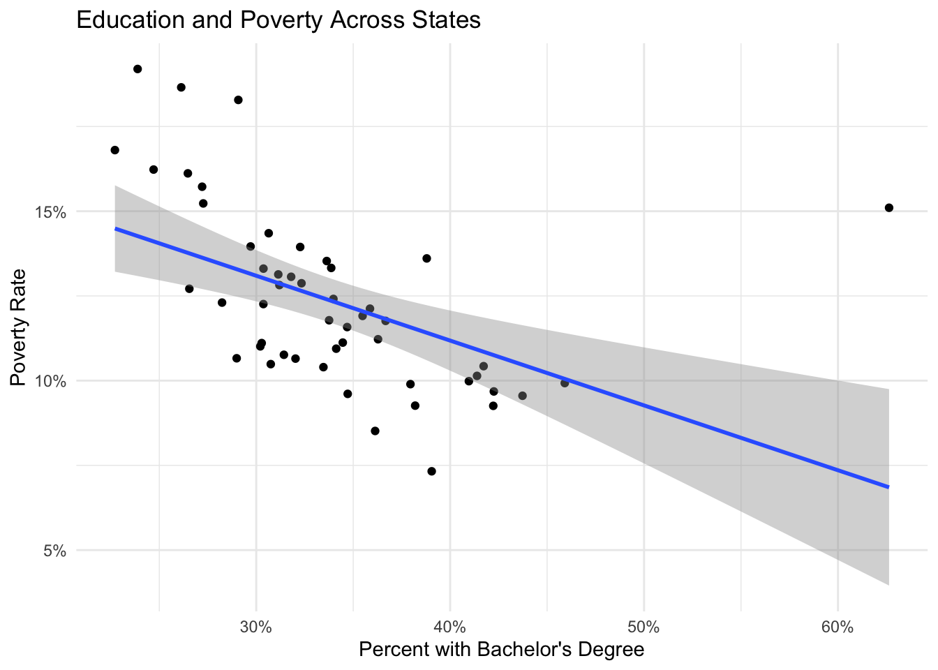
8.12 Exercises
8.12.1 Linear Regression
Using the state data, regress median rent on median household income and homeownership rate. Interpret the coefficients and R-squared.
Estimate a Mincer wage equation using the PUMS data that includes education, experience, experience-squared, sex, and state fixed effects. Calculate the return to an additional year of education.
Using the macro data, estimate the relationship between real GDP per capita and the unemployment rate (Okun’s Law). Include a time trend. Plot the results.
Test whether the relationship between education and income differs by region. Estimate a model with region dummy variables and interaction terms.
8.12.2 Binary Response Models
Using the PUMS data, estimate a probit model for homeownership (tenure == “Owner”) as a function of age, household income, education, and marital status. Calculate marginal effects.
Compare logit and probit models for the employment probability regression. Are the predicted probabilities similar?
Create a visualization showing how the predicted probability of homeownership varies with household income for different education levels.
8.12.3 Count Data Models
Using the cafe data, estimate a Poisson regression for daily transaction counts as a function of day of week, month, and year. Test for overdispersion.
Compare Poisson, quasi-Poisson, and negative binomial models for the cafe transaction data. Which fits best?
Using the PUMS data, model the number of children (
num_children) as a function of age, education, marital status, and household income using Poisson regression.
8.12.4 Model Comparison and Diagnostics
For the state income regression, create diagnostic plots and identify any outliers or influential observations. How do results change if you exclude them?
Estimate three nested models predicting state median income with progressively more variables. Use likelihood ratio tests and information criteria to compare them.
Calculate robust standard errors for the wage regression. How much do the standard errors change?
8.12.5 Advanced
Estimate an augmented Phillips curve that includes lagged inflation (inflation expectations). Interpret the results.
Create a publication-ready regression table comparing at least three model specifications for an outcome of your choice, including coefficient estimates, standard errors, and fit statistics.